3. Tutorial

AirfoilPrep.py can be accessed either through the command line or through Python. The command-line interface is the simplest but provides only a limited number of options. The Python interface is useful for more advanced preprocessing and for integration with other codes.

3.1. Command-Line Usage

From the terminal, to see the options, invoke help:

$ python airfoilprep.py -h

When using the command-line options, all files must be AeroDyn formatted files. The command line provides three main methods for working with files directly: 3-D stall corrections, high angle of attack extrapolation, and a blending operation. In all cases, you first specify the name (and path if necessary) of the file you want to work with:

$ python airfoilprep.py airfoil.dat

The following optional arguments are available

Available Flags

flag	arguments	description
-h		display help
--stall3D	r/R c/r tsr	3-D rotational corrections near stall
--extrap	cdmax	high angle of attack extrapolation
--blend	other weight	blend with other file using specified weight
--out	outfile	specify a different name for output file
--plot		plot data (for diagnostic purposes) using matplotlib
--common		output airfoil data using a common set of angles of attack

3.1.1. Stall Corrections

The first method available from the command line is --stall3D, which reads the file, applies rotational corrections, and then writes the data to a separate file. This argument must specify the parameters used for the correction in the format --stall3D r/R c/r tsr, where r/R is the local radius normalized by the rotor radius, c/r is the local chord normalized by the local radius, and tsr is the local tip-speed ratio. For example, if airfoil.dat contained 2-D data with r/R=0.5, c/r=0.15, tsr=5.0, then we would apply rotational corrections to the airfoil using:

$ python airfoilprep.py airfoil.dat --stall3D 0.5 0.15 5.0

By default the output file will append _3D to the name. In the above example, the output file would be airfoil_3D.dat. However, this can be overriden with the --out option. To output to a file at /Users/Me/Airfoils/my_new_airfoil.dat:

$ python airfoilprep.py airfoil.dat --stall3D 0.5 0.15 5.0 \
> --out /Users/Me/Airfoils/my_new_airfoil.dat

Optionally, you can also plot the results (matplotlib must be installed) with the --plot flag. For example,

$ python airfoilprep.py DU21_A17.dat --stall3D 0.2 0.3 5.0 --plot

displays Figure 1 (only one Reynolds number shown) along with producing the output file.

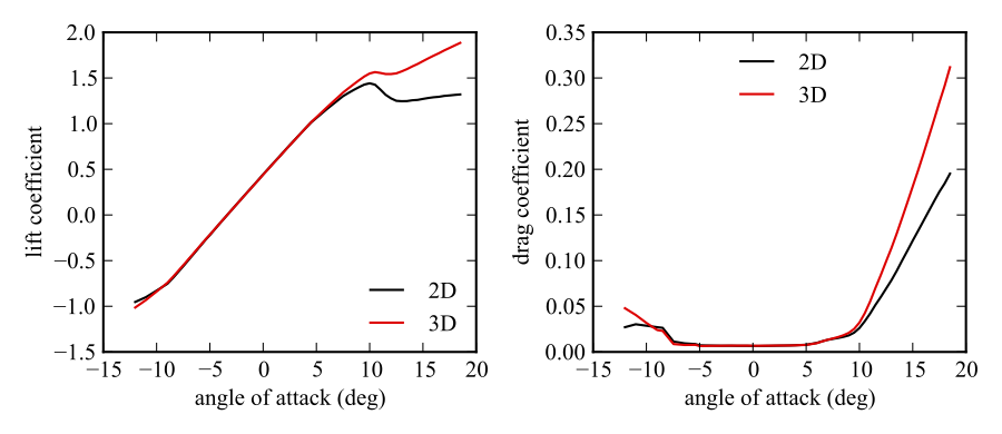
Figure 1: Lift and drag coefficient with 3-D stall corrections applied.

AirfoilPrep.py can utilize data for which every Reynolds number uses a different set of angles of attack. However, some codes need data on a uniform grid of Reynolds number and angle of attack. To output the data on a common set of angles of attack, use the --common flag.

$ python airfoilprep.py airfoil.dat --stall3D 0.5 0.15 5.0 --common

3.1.2. Angle of Attack Extrapolation

The second method available from the command line is --extrap, which reads the file, applies high angle of attack extrapolations, and then writes the data to a separate file. This argument must specify the maximum drag coefficient to use in the extrapolation across the full +/- 180-degree range --extrap cdmax. For example, if airfoil_3D.dat contained 3D stall corrected data and cdmax=1.3, then we could extrapolate the airfoil using:

$ python airfoilprep.py airfoil_3D.dat --extrap 1.3

By default the output file will append _extrap to the name. In the above example, the output file would be airfoil_3D_extrap.dat. However, this can also be overriden with the --out flag. The --common flag is also useful here if a common set of angles of attack is needed.

The output can be plotted with the –plot flag. The command

$ python airfoilprep.py DU21_A17_3D.dat --extrap 1.3 --plot

displays Figure 2 (only one Reynolds number shown) along with producing the output file.

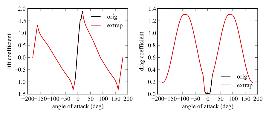
Figure 2: Airfoil data extrapolated to high angles of attack.

3.1.3. Blending

The final capability accessible from the command line is blending of airfoils. This is invoked through --blend filename weight, where filename is the name (and path if necessary) of a second file to blend with, and weight is the weighting used in the blending. The weight ranges on a scale of 0 to 1 where 0 returns the first airfoil and 1 the second airfoil. For example, the following command blends airfoil1.dat with airfoil2.dat with a weighting of 0.3 (conceptually the new airfoil would equal 0.7*airfoil1.dat + 0.3*airfoil2.dat).

$ python airfoilprep.py airfoil1.dat --blend airfoil2.dat 0.3

By default, the output file appends the names of the two files with a ‘+’ sign, then appends the weighting using ‘_blend’ and the value for the weight. In this example, the output file would be airfoil1+airfoil2_blend0.3.dat. Just like the previous case, the name of the output file can be overridden by using the --out flag. The --common flag is also useful here if a common set of angles of attack is needed. This data can also be plotted, but only the blended airfoil data will be shown. Direct comparison to the original data is not always possible, because the blend method allows for the specified airfoils to be defined at different Reynolds numbers. Blending first occurs across Reynolds numbers and then across angle of attack.

3.2. Python Usage

The Python interface allows for more flexible usage or integration with other programs. Descriptions of the interfaces for the classes contained in the module are contained in Module Documentation.

Airfoils can be created from AeroDyn formatted files,

from airfoilprep import Polar, Airfoil
import numpy as np

airfoil = Airfoil.initFromAerodynFile('DU21_A17.dat')

or they can be created directly from airfoil data.

# first polar
Re = 7e6
alpha = [-14.50, -12.01, -11.00, -9.98, -8.12, -7.62, -7.11, -6.60, -6.50,
         -6.00, -5.50, -5.00, -4.50, -4.00, -3.50, -3.00, -2.50, -2.00, -1.50,
         -1.00, -0.50, 0.00, 0.50, 1.00, 1.50, 2.00, 2.50, 3.00, 3.50, 4.00,
         4.50, 5.00, 5.50, 6.00, 6.50, 7.00, 7.50, 8.00, 8.50, 9.00, 9.50,
         10.00, 10.50, 11.00, 11.50, 12.00, 12.50, 13.00, 13.50, 14.00, 14.50,
         15.00, 15.50, 16.00, 16.50, 17.00, 17.50, 18.00, 18.50, 19.00, 19.50,
         20.00, 20.50]
cl = [-1.050, -0.953, -0.900, -0.827, -0.536, -0.467, -0.393, -0.323, -0.311,
      -0.245, -0.178, -0.113, -0.048, 0.016, 0.080, 0.145, 0.208, 0.270, 0.333,
      0.396, 0.458, 0.521, 0.583, 0.645, 0.706, 0.768, 0.828, 0.888, 0.948,
      0.996, 1.046, 1.095, 1.145, 1.192, 1.239, 1.283, 1.324, 1.358, 1.385,
      1.403, 1.401, 1.358, 1.313, 1.287, 1.274, 1.272, 1.273, 1.273, 1.273,
      1.272, 1.273, 1.275, 1.281, 1.284, 1.296, 1.306, 1.308, 1.308, 1.308,
      1.308, 1.307, 1.311, 1.325]
cd = [0.0567, 0.0271, 0.0303, 0.0287, 0.0124, 0.0109, 0.0092, 0.0083, 0.0089,
      0.0082, 0.0074, 0.0069, 0.0065, 0.0063, 0.0061, 0.0058, 0.0057, 0.0057,
      0.0057, 0.0057, 0.0057, 0.0057, 0.0057, 0.0058, 0.0058, 0.0059, 0.0061,
      0.0063, 0.0066, 0.0071, 0.0079, 0.0090, 0.0103, 0.0113, 0.0122, 0.0131,
      0.0139, 0.0147, 0.0158, 0.0181, 0.0211, 0.0255, 0.0301, 0.0347, 0.0401,
      0.0468, 0.0545, 0.0633, 0.0722, 0.0806, 0.0900, 0.0987, 0.1075, 0.1170,
      0.1270, 0.1368, 0.1464, 0.1562, 0.1664, 0.1770, 0.1878, 0.1987, 0.2100]

p1 = Polar(Re, alpha, cl, cd)

# second polar
Re = 9e6
alpha = [-14.24, -13.24, -12.22, -11.22, -10.19, -9.70, -9.18, -8.18, -7.19,
         -6.65, -6.13, -6.00, -5.50, -5.00, -4.50, -4.00, -3.50, -3.00, -2.50,
         -2.00, -1.50, -1.00, -0.50, 0.00, 0.50, 1.00, 1.50, 2.00, 2.50, 3.00,
         3.50, 4.00, 4.50, 5.00, 5.50, 6.00, 6.50, 7.00, 7.50, 8.00, 9.00,
         9.50, 10.00, 10.50, 11.00, 11.50, 12.00, 12.50, 13.00, 13.50, 14.00,
         14.50, 15.00, 15.50, 16.00, 16.50, 17.00, 17.50, 18.00, 18.50, 19.00]
cl = [-1.229, -1.148, -1.052, -0.965, -0.867, -0.822, -0.769, -0.756, -0.690,
      -0.616, -0.542, -0.525, -0.451, -0.382, -0.314, -0.251, -0.189, -0.120,
      -0.051, 0.017, 0.085, 0.152, 0.219, 0.288, 0.354, 0.421, 0.487, 0.554,
      0.619, 0.685, 0.749, 0.815, 0.879, 0.944, 1.008, 1.072, 1.135, 1.197,
      1.256, 1.305, 1.390, 1.424, 1.458, 1.488, 1.512, 1.533, 1.549, 1.558,
      1.470, 1.398, 1.354, 1.336, 1.333, 1.326, 1.329, 1.326, 1.321, 1.331,
      1.333, 1.340, 1.362]
cd = [0.1461, 0.1263, 0.1051, 0.0886, 0.0740, 0.0684, 0.0605, 0.0270, 0.0180,
      0.0166, 0.0152, 0.0117, 0.0105, 0.0097, 0.0092, 0.0091, 0.0089, 0.0089,
      0.0088, 0.0088, 0.0088, 0.0088, 0.0088, 0.0087, 0.0087, 0.0088, 0.0089,
      0.0090, 0.0091, 0.0092, 0.0093, 0.0095, 0.0096, 0.0097, 0.0099, 0.0101,
      0.0103, 0.0107, 0.0112, 0.0125, 0.0155, 0.0171, 0.0192, 0.0219, 0.0255,
      0.0307, 0.0370, 0.0452, 0.0630, 0.0784, 0.0931, 0.1081, 0.1239, 0.1415,
      0.1592, 0.1743, 0.1903, 0.2044, 0.2186, 0.2324, 0.2455]
p2 = Polar(Re, alpha, cl, cd)

# create airfoil object (can contain as many polars as desired)
af = Airfoil([p1, p2])

Blending is easily accomplished just like in the command-line interface. There is no requirement that the two airfoils share a common set of angles of attack.

airfoil1 = Airfoil.initFromAerodynFile('DU21_A17.dat')
airfoil2 = Airfoil.initFromAerodynFile('DU25_A17.dat')

# blend the two airfoils
airfoil_blend = airfoil1.blend(airfoil2, 0.3)

Applying 3-D corrections and high alpha extensions directly in Python, allows for a few additional options as compared to the command-line version. The following example performs the same 3-D correction as in the command-line version, followed by an alternative 3-D correction that utilizes some of the optional inputs. See correction3D for more details on the optional parameters.

r_over_R = 0.5
chord_over_r = 0.15
tsr = 5.0

# 3D stall correction
af3D_ex1 = af.correction3D(r_over_R, chord_over_r, tsr)

# a second example using the optional inputs
alpha_max_corr = 25  # apply full rotational correction only up to this angle of attack
alpha_linear_min = -3  # angle of attack to start evaluating slope of linear region
alpha_linear_max = 7  # angle of attack to stop evaluating slope of linear region

af3D_ex2 = af.correction3D(r_over_R, chord_over_r, tsr,
                           alpha_max_corr=alpha_max_corr,
                           alpha_linear_min=alpha_linear_min,
                           alpha_linear_max=alpha_linear_max)

The airfoil data can be extended to high angles of attack using the extrapolate method. Just like the previous method, a few optional parameters are available through the Python interface. The following example performs the same extrapolation as in the command-line version, followed by an alternative extrapolation that utilizes some of the optional inputs.

cdmax = 1.3

# compute a 3D corrected and extended airfoil
af_extrap1 = af.extrapolate(cdmax)

# a second example using the optional inputs
AR = 17  # blade aspect ratio. If provided, cdmax is estimated using the aspect ratio.
cdmin = 0.001  # minimum drag coefficient.  Viterna's method can occasionally produce
               # negative drag coefficients.  A minimum is used to prevent unphysical data.
               # The passed in value is used to override the default.

af_extrap2 = af.extrapolate(cdmax, AR=AR, cdmin=cdmin)

Some codes need to use the same set of angles of attack data for every Reynolds number defined in the airfoil. The following example performs the same method as in the command-line version followed by an alternate approach where the user can specify the set of angles of attack to use.

# create new airfoil that uses the same angles of attack at each Reynolds number
af_common1 = af.interpToCommonAlpha()

# default approach uses a union of all defined angles of attack
# alternatively, specify the exact angles to use
alpha = np.arange(-180, 180)
af_common2 = af.interpToCommonAlpha(alpha)

For direct access to the underlying data in a grid format (if not already a grid, it is interpolated to a grid first), use the createDataGrid method as follows:

# extract a data grid from airfoil
alpha, Re, cl, cd = af.createDataGrid()

# cl[i, j] is the lift coefficient for alpha[i] and Re[j]

Finally, writing AeroDyn formatted files is straightforward.

af.writeToAerodynFile('output.dat')