5. Theory

The methodology details are available in Yang [Yan86]. Usage differs here only in that rather than using precomputed matrices for an assumed variation in structural properties, a polynomial representation is assumed that allows for more flexible usage and exact polynomial integration.

Nomenclature

symbol	definition
\(K\)	stiffness matrix
\(M\)	inertia matrix or moment
\(N\)	incremental stiffness matrix
\(q\)	displacement vector
\(F\)	force vector
\(\eta\)	nondimensional coordinate along element
\(L\)	length of element
\(\rho\)	mass density
\(m\)	mass
\(A\)	cross-sectional area
\(I\)	area moment of inertia
\(J\)	polar area moment of inertia
\(E\)	modulus of elasticity
\(G\)	shear modulus of elasticity
\(f\)	shape function
\(v\)	velocity vector
\(\omega\)	angular velocity vector
\(V\)	shear force

5.1. Finite Element Matrices

The governing equation of the structure is given by

\[Kq + M\ddot{q} = F\]

and for buckling analysis

\[[K - N]q = F\]

The finite element matrices are computed from the structural properties of the beam. As mentioned earlier, pBEAM uses a polynomial representation of the structural properties. All polynomials are defined across an element in normalized coordinates (\(\eta\)). For example, the moment of inertia across an element may vary quadratically as \(I_2 \eta^2 + I_1 \eta + I_0\). Computation of the finite element matrices are described below, where all derivatives are with respect to \(\eta\).

bending stiffness matrix:

\[K_{ij} = \frac{1}{L^3} \int_0^1 EI(\eta) f_i^{\prime\prime}(\eta) f_j^{\prime\prime}(\eta) d\eta\]

bending inertia matrix:

\[M_{ij} = L \int_0^1 \rho A(\eta) f_i(\eta) f_j(\eta) d\eta\]

incremental stiffness matrix:

\[N_{ij} = \frac{1}{L} \int_0^1 F_z(\eta) f_i^\prime(\eta) f_j^\prime(\eta) d\eta\]

axial stiffness matrix:

\[K_{ij} = \frac{1}{L} \int_0^1 EA(\eta) f_i^{\prime}(\eta) f_j^{\prime}(\eta) d\eta\]

axial inertia matrix:

\[M_{ij} = L \int_0^1 \rho A(\eta) f_i(\eta) f_j(\eta) d\eta\]

Torsional matrices are computed similarly to the axial matrices, except \(EA(\eta)\) is replaced with \(GJ(\eta)\) and \(\rho A(\eta)\) is replaced with \(\rho J(\eta)\). Note that although the same notation was used, the axial shape functions are not the same as those for bending. Because section properties are defined as polynomials, each of these derivatives and integrals are done analytically.

5.2. Top Mass

pBEAM assumes that the top of the beam is a free end, but that a mass may exist on top of the beam. This is useful for modeling structures such as an RNA (rotor/nacelle/assembly) on top of a wind turbine tower. The top mass is assumed to be a rigid body with respect to the main beam and thus, does not contribute to the stiffness matrix. It does, however, affect the inertial loading and external forces as discussed below. The top mass can be offset from the beam top by some vector \(\rho\). Although idealized as a point mass, its moment of inertia matrix can also be specified. The tip is both translating and rotating, so the velocity of the tip mass in an inertial reference frame is given by (with reference to the variables in Figure 1):

\[\vec{v}_m = \frac{d\vec{r}}{dt} + \left(\frac{\vec{d \rho}}{dt}\right)_\rho + \vec{\omega} \times \vec{\rho}\]

where the second time derivative is taken in the rotating reference frame. The kinetic energy of the mass is then

\[\begin{split}T &= \frac{1}{2} m \vec{v}_m \cdot \vec{v}_m + \frac{1}{2} \vec{\omega}^T I \vec{\omega} \\ &= \frac{1}{2} m \left[ (\dot{x} + \dot{\theta_y} \rho_z - \dot{\theta_z}\rho_y)^2 + (\dot{y} + \dot{\theta_z} \rho_x - \dot{\theta_x}\rho_z)^2 + (\dot{z} + \dot{\theta_x} \rho_y - \dot{\theta_y}\rho_x)^2 \right] \\ &+ \frac{1}{2} \left[ I_{xx} \dot{\theta_x}^2 + 2 I_{xy} \dot{\theta_x}\dot{\theta_y} + 2 I_{xz}\dot{\theta_x}\dot{\theta_z} + \dots \right]\end{split}\]

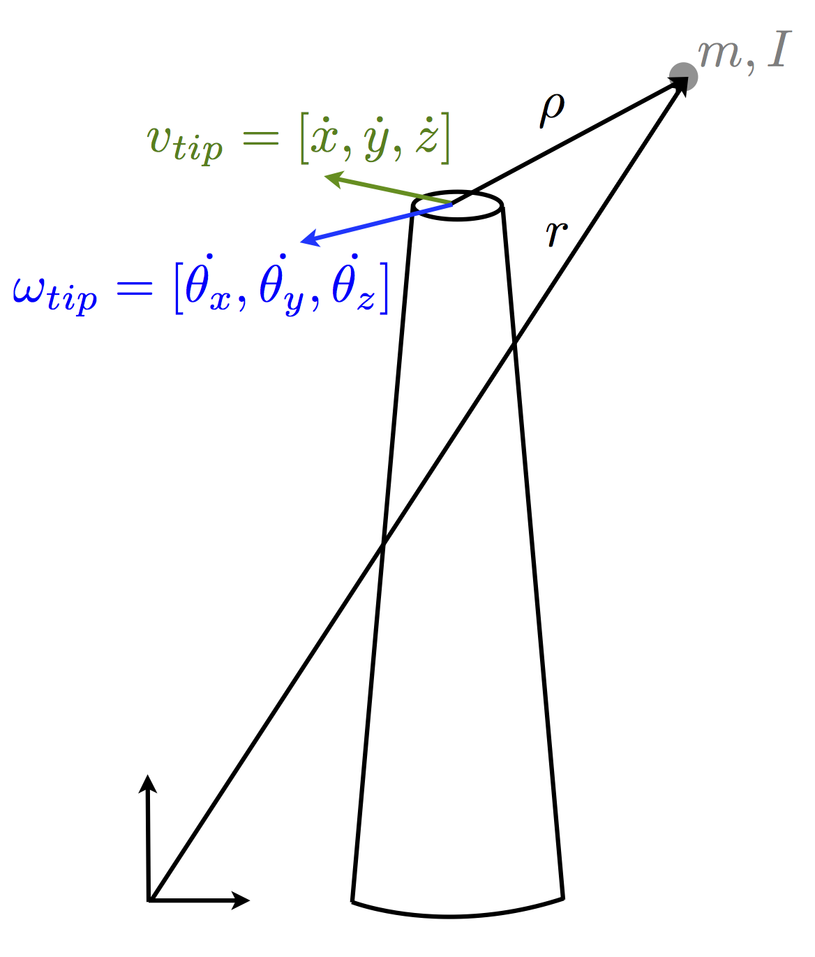
Figure 1: Diagram of top mass idealized as a point mass with moments of inertia. The center of mass of the top mass is offset by vector \(\rho\) relative to the top of the beam. The top of the beam is also potentially translating and rotating.

Using the Lagrangian one can show that

\[(M \ddot{q})_i = \frac{d}{dt} \frac{\partial T}{\partial \dot{q_i}}\]

After taking the derivatives, the inertial matrix contribution from the top mass is given by

\[\begin{split}M_{tip} = \left[ \begin{array}{cccccc} m & & & m\rho_z & & -m\rho_y \\ & I_{xx} + m (\rho_y^2 +\rho_z^2) & -m\rho_z & I_{xy} - m\rho_x\rho_y& m\rho_y & I_{xz}-m\rho_x\rho_z \\ & -m\rho_z & m & && m\rho_x \\ m\rho_z & I_{xy}-m\rho_x\rho_y & & I_{yy} + m(\rho_x^2+\rho_z^2)& -m\rho_x& I_{yz}-m\rho_y\rho_z \\ & m\rho_y & & -m\rho_x& m & \\ -m\rho_y & I_{xz}-m\rho_x\rho_z & m\rho_x & I_{yz}-m\rho_y\rho_z& & I_{zz} + m(\rho_x^2+\rho_y^2) \\ \end{array} \right]\end{split}\]

where \(q = [x,\theta_x,y,\theta_y,z,\theta_z]\). Note that the current implementation assumes moments of inertia are given about the beam tip, though moments of inertia about its own center of mass are easily translated to the beam tip via the generalized parallel axis theorem.

Finally, the top mass may also apply loads (forces and moments) to the beam. These are simply added to the force vector at the tip of the structure. It is assumed that the weight of the top mass was already added to the force vector.

5.3. Base

The bottom of the beam is assumed to be constrained by linear springs in all 6 coordinate directions. Any of these springs can be chosen to be infinitely stiff, or in other words, rigidly constrained in that direction. This simply adds a diagonal stiffness matrix at the bottom of the beam, and directions that are rigid are removed from the structural matrices.

5.4. Loads

Distributed loads, point forces, and point moments can be specified anywhere in the structure. Distributed loads are specified as polynomials across the elements. For distributed loads in the lateral directions, work equivalent loads are computed at the nodes. Axially distributed loads are integrated starting from the free end of the beam to compute the polynomial variation in axial force.

5.5. Axial Stress

The computation of axial stress is separate from the finite element analysis, but is included in this code for convenience. First, the forces and moments must be computed along the beam. For example the shear force and moments are evaluated as

\[\begin{split}V_i &= V_{i+1}(0) + {F_{pt}}_{i+1} + (z_{i+1}-z_i) \int_{1}^0 q(\eta) d\eta \\ M_i &= M_{i+1}(0) + {M_{pt}}_{i+1} + (z_{i+1}-z_i) \int_{1}^0 V_i(\eta) d\eta\end{split}\]

where \(F_{pt}\) and \(M_{pt}\) are external point forces and moments along the structure. Note that the integration is actually an indefinite integral, but limits are noted to signify that integration must be done from the tip where forces/moments are known. Finally, the stress is computed as (or use \(E(x, y) = 1\) to compute strain):

\[\sigma_{zz}(x, y) = E(x, y) \left(\frac{M_x}{[EI]_x} y - \frac{M_y}{[EI]_y} x + \frac{N_z}{[EA]} \right)\]

Bibliography

[Han08]

Martin O. L. Hansen. Aerodynamics of Wind Turbines. Earthscan, 2nd edition, 2008.

[Yan86]

T. Y. Yang. Finite Element Structural Analysis. Prentice Hall College Div, 1986.