3. Tutorial
Two examples are included in this section. The first example provides the sectional properties and assumes a linear variation between the sections (see matching constructor). The example simulates a blade for the NREL 5-MW reference model. The second example uses the convenience constructor for a beam with cylindrical shell sections (see matching constructor). The example simulates the tower for the NREL 5-MW refernece model. A third constructor is available for more advanced usage and allows for arbitrary polynomial variation in section properties. This advanced constructor is not demonstrated in these examples, but details are available in the :ref:`documentation <documentation-label>.
3.1. Linear Variation
This example simulates a rotor blade from the NREL 5-MW reference model in pBEAM. First, the relevant modules are imported.
import numpy as np
import matplotlib.pyplot as plt

import _pBEAM
Next, we define the stiffness and inertial properties. The stiffness and inertial properties can be computed from the structural layout of the blade using a code like PreComp. Section properties are defined using the SectionData class.
# stiffness / inertial properties

r = np.array([1.501, 1.803, 1.902, 2, 2.105, 2.203, 2.302, 2.868, 3.003, 3.102,
              5.607, 7.005, 8.34, 10.51, 11.76, 13.51, 15.86, 18.52, 19.97,
              22.02, 24.07, 26.12, 28.17, 32.28, 33.53, 36.39, 38.53, 40.49,
              42.54, 43.54, 44.59, 46.54, 48.7, 52.8, 56.22, 58.95, 61.69, 63.06])
EA = np.array([1.626e+10, 1.65e+10, 1.677e+10, 1.685e+10, 1.694e+10, 1.702e+10,
               1.625e+10, 1.208e+10, 1.212e+10, 1.23e+10, 1.228e+10, 1.199e+10,
               1.16e+10, 8.27e+09, 8.035e+09, 8.42e+09, 8.754e+09, 8.972e+09,
               9.058e+09, 9.128e+09, 9.122e+09, 8.947e+09, 8.747e+09, 8.295e+09,
               8.088e+09, 7.532e+09, 7.09e+09, 6.645e+09, 6.079e+09, 5.809e+09,
               5.515e+09, 4.955e+09, 4.353e+09, 3.186e+09, 2.221e+09, 1.503e+09,
               9.426e+08, 7.459e+08])
EI11 = np.array([2.352e+10, 2.352e+10, 2.491e+10, 2.491e+10, 2.491e+10, 2.491e+10,
                 2.372e+10, 1.659e+10, 1.751e+10, 1.821e+10, 1.456e+10, 1.336e+10,
                 1.065e+10, 4.918e+09, 4.769e+09, 4.331e+09, 4.044e+09, 3.423e+09,
                 3.167e+09, 2.873e+09, 2.572e+09, 1.969e+09, 1.58e+09, 1.296e+09,
                 1.101e+09, 7.37e+08, 6.386e+08, 5.837e+08, 4.358e+08, 3.622e+08,
                 3.096e+08, 2.541e+08, 2.034e+08, 1.22e+08, 7.101e+07, 3.817e+07,
                 7.727e+06, 3.664e+06])
EI22 = np.array([2.307e+10, 2.307e+10, 2.328e+10, 2.328e+10, 2.328e+10, 2.328e+10,
                 2.217e+10, 1.555e+10, 1.524e+10, 1.495e+10, 1.848e+10, 1.69e+10,
                 1.342e+10, 6.219e+09, 5.231e+09, 5.255e+09, 5.286e+09, 4.943e+09,
                 4.699e+09, 4.421e+09, 4.142e+09, 3.674e+09, 3.241e+09, 2.603e+09,
                 2.397e+09, 1.995e+09, 1.756e+09, 1.558e+09, 1.292e+09, 1.215e+09,
                 1.107e+09, 9.199e+08, 7.931e+08, 5.797e+08, 4.296e+08, 3.009e+08,
                 9.361e+07, 4.69e+07])
GJ = np.array([1.079e+10, 1.128e+10, 1.182e+10, 1.199e+10, 1.217e+10, 1.234e+10,
               1.192e+10, 8.915e+09, 9.135e+09, 9.261e+09, 7.303e+09, 4.995e+09,
               2.821e+09, 5.891e+08, 4.595e+08, 4.022e+08, 3.556e+08, 2.913e+08,
               2.697e+08, 2.414e+08, 2.157e+08, 1.689e+08, 1.415e+08, 1.191e+08,
               1.019e+08, 7.086e+07, 6.037e+07, 5.437e+07, 4.033e+07, 3.455e+07,
               3.002e+07, 2.53e+07, 2.128e+07, 1.433e+07, 9.588e+06, 6.455e+06,
               4.335e+06, 3.017e+06])
rhoA = np.array([1086, 1102, 1121, 1126, 1132, 1137, 1086, 878.6, 891.2, 896.1,
                 730.2, 608.9, 559.4, 337.1, 332.3, 333.3, 331.2, 324.2, 320.7,
                 315, 308, 271.6, 261.2, 244.8, 237, 218.2, 206.2, 194.8, 157,
                 151, 144.5, 133.1, 122.1, 100.6, 82.32, 67.6, 46.81, 31.18])
rhoJ = np.array([2778, 2905, 3048, 3092, 3139, 3184, 3075, 2415, 2532, 2566,
                 2119, 1595, 1255, 576.9, 558, 554.2, 534, 488.8, 467.5, 436.7,
                 404.6, 331.1, 295.2, 243.2, 222.8, 180.2, 155.6, 135.1, 92.91,
                 85.2, 76.85, 63.57, 52.86, 35.45, 23.82, 16.32, 8.66, 6.038])


# number of sections
nsec = len(r)

p_section = _pBEAM.SectionData(nsec, r, EA, EI11, EI22, GJ, rhoA, rhoJ)
Distributed loads can be computed from an aerodynamics code like CCBlade. This example includes only distributed loads, which are defined in Loads.
# distributed loads

P1 = np.array([106.8, 487.3, 604.7, 715.4, 826.2, 923.1, 1007, 1299, 1326,
               1343, 1440, 1337, 1108, -1252, -2185, -2017, -1736, -1727,
               -1718, -1698, -1665, -1419, -1131, -1051, -937, -673.4,
               -643.8, -617, -553.7, -524.2, -504.1, -484.4, -462.8,
               -417, -374.3, -336.6, -295.3, -0.01844])
P2 = np.array([452.4, 2064, 2561, 3030, 3499, 3909, 4263, 5499, 5612,
               5686, 6098, 5291, 4690, 1.938e+04, 2.563e+04, 2.492e+04,
               2.387e+04, 2.346e+04, 2.308e+04, 2.202e+04, 2.097e+04,
               2.021e+04, 1.959e+04, 1.865e+04, 1.844e+04, 1.796e+04,
               1.734e+04, 1.668e+04, 1.592e+04, 1.556e+04, 1.518e+04,
               1.452e+04, 1.379e+04, 1.23e+04, 1.096e+04, 9802, 8552,
               13.34])
P3 = np.array([-1.065e+04, -1.081e+04, -1.098e+04, -1.104e+04, -1.109e+04,
               -1.114e+04, -1.064e+04, -8611, -8734, -8782, -7156, -5967,
               -5482, -3303, -3256, -3267, -3246, -3177, -3143, -3087,
               -3019, -2662, -2560, -2399, -2323, -2138, -2021, -1909,
               -1539, -1480, -1416, -1305, -1197, -985.7, -806.8, -662.5,
               -458.7, -305.5])


p_loads = _pBEAM.Loads(nsec, P1, P2, P3)  # only distributed loads
The tip/base data is defined with a free end in TipData and a rigid base for BaseData. The blade object is then assembled using the Beam constructor that assumes linear variation in properties between sections.
# tip/base data
p_tip = _pBEAM.TipData()  # no tip mass
k = np.array([float('inf'), float('inf'), float('inf'),
              float('inf'), float('inf'), float('inf')])
p_base = _pBEAM.BaseData(k, float('inf'))  # rigid base

# create blade object
blade = _pBEAM.Beam(p_section, p_loads, p_tip, p_base)
The constructed blade object can now be used for various computations. For example, the mass and the first five natural frequencies
# compute mass and natural frequncies
print 'mass =', blade.mass()
print 'natural freq =', blade.naturalFrequencies(5)
which result in
>>> mass = 17170.0189
>>> natural freq = [ 0.90910346  1.13977516  2.81855826  4.23836926  6.40037864]
Figure 1 shows a plot of the blade displacement in the second principal direction generated from the following commands.
# plot displacement in second principal direction (approximately flapwise direction)
disp = blade.displacement()
dy = disp[1]
plt.plot(r, dy)
plt.xlabel('r (m)')
plt.ylabel('$\delta y$ (m)')
# plt.show()
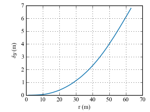
Figure 1: Blade deflection along span in flapwise direction.
Figure 2 shows a plot of the strain along the blade at the location of maximum airfoil thickness on both the pressure and suction side of the airfoil.
# evaluate strain at location of max airfoil thickness (upper and lower surface)
xpt = np.array([-0.02676, -0.02716, 0.009337, 0.009381, 0.009428, 0.009472,
                0.009515, -0.02336, 0.01155, 0.01219, -0.1379, -0.2207, -0.4827,
                -0.5969, -0.63, -0.6355, -0.6947, -0.6163, -0.6085, -0.5971,
                -0.5857, -0.5064, -0.4283, -0.3977, -0.3872, -0.3107, -0.2956,
                -0.2811, -0.212, -0.2087, -0.2012, -0.1864, -0.1791, -0.1669,
                -0.1599, -0.1587, -0.1586, -0.1559, -0.02725, -0.02765, 0.00883,
                0.008872, 0.008916, 0.008958, 0.008999, -0.02389, 0.01102,
                0.01165, -0.1384, -0.2211, -0.4831, -0.5972, -0.6303, -0.6357,
                -0.695, -0.6165, -0.6088, -0.5973, -0.5859, -0.5066, -0.4285,
                -0.3979, -0.3874, -0.3108, -0.2957, -0.2813, -0.2121, -0.2088,
                -0.2013, -0.1865, -0.1792, -0.167, -0.16, -0.1588, -0.1586, -0.1559])
ypt = np.array([1.63, 1.654, 1.686, 1.694, 1.702, 1.71, 1.718, 1.738, 1.773, 1.779,
                1.665, 1.465, 1.253, 0.9807, 0.8931, 0.8325, 0.7735, 0.7064, 0.6822,
                0.6488, 0.6125, 0.545, 0.4985, 0.4701, 0.4415, 0.3727, 0.354,
                0.3417, 0.3047, 0.2843, 0.2697, 0.2551, 0.2419, 0.2138, 0.1895,
                0.1694, 0.1488, 0.1382, -1.63, -1.654, -1.686, -1.694, -1.703,
                -1.711, -1.718, -1.738, -1.774, -1.78, -1.674, -1.482, -1.287,
                -1.022, -0.9412, -0.89, -0.8412, -0.7795, -0.7559, -0.7211, -0.6782,
                -0.5917, -0.5272, -0.4972, -0.4647, -0.3841, -0.3647, -0.3522,
                -0.3056, -0.2824, -0.2651, -0.2505, -0.2371, -0.208, -0.1823,
                -0.1605, -0.137, -0.1247])
zpt = np.array([1.501, 1.803, 1.902, 2, 2.105, 2.203, 2.302, 2.868, 3.003, 3.102,
                5.607, 7.005, 8.34, 10.51, 11.76, 13.51, 15.86, 18.52, 19.97,
                22.02, 24.07, 26.12, 28.17, 32.28, 33.53, 36.39, 38.53, 40.49,
                42.54, 43.54, 44.59, 46.54, 48.7, 52.8, 56.22, 58.95, 61.69,
                63.06, 1.501, 1.803, 1.902, 2, 2.105, 2.203, 2.302, 2.868, 3.003,
                3.102, 5.607, 7.005, 8.34, 10.51, 11.76, 13.51, 15.86, 18.52,
                19.97, 22.02, 24.07, 26.12, 28.17, 32.28, 33.53, 36.39, 38.53,
                40.49, 42.54, 43.54, 44.59, 46.54, 48.7, 52.8, 56.22, 58.95,
                61.69, 63.06])

strain = blade.axialStrain(len(xpt), xpt, ypt, zpt)
nstrain = len(strain)/2
plt.figure()
plt.plot(r, strain[:nstrain], label='suction side')
plt.plot(r, strain[nstrain:], label='pressure side')
plt.xlabel('r (m)')
plt.ylabel('$\epsilon$')
plt.legend()
plt.xlim([0, 63.0])
# plt.show()
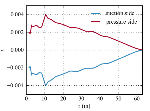
Figure 2: Strain along span at location of maximum airfoil thickness.
3.2. Cylindrical Shell Sections
This example simulates the tower from the NREL 5-MW reference model in pBEAM. First, the relevant modules are imported
import numpy as np
from math import pi
import matplotlib.pyplot as plt

import _pBEAM
The basic tower geometry is defined
# tower geometry defintion
z0 = [0, 30.0, 73.8, 117.6]             # heights starting from bottom (m)
d0 = [6.0, 6.0, 4.935, 3.87]            # corresponding diameters (m)
t0 = [0.0351, 0.0351, 0.0299, 0.0247]   # corresponding shell thicknesses (m)
n0 = [5, 5, 5]                          # number of finite elements per section
and then discretized so that it is defined at the end of every element (for convenience, a discretized definition could be supplied up front).
# discretize
nodes = int(np.sum(n0)) + 1  # C++ interface requires int

z = np.zeros(nodes)
start = 0
for i in range(len(n0)):
    z[start:start+n0[i]+1] = np.linspace(z0[i], z0[i+1], n0[i]+1)
    start += n0[i]

d = np.interp(z, z0, d0)
t = np.interp(z, z0, t0)
The cylindrical shell model only allows for isotropic material properties.
# material properties

E = 210e9               # elastic modulus (Pa)
G = 80.8e9              # shear modulus (Pa)
rho = 8500.0            # material density (kg/m^3)

material = _pBEAM.Material(E, G, rho)
Distributed loads in this example come from wind loading and the tower’s weight.
# distributed loads

g = 9.81  # gravity

# wind loading in x-direction
Px = np.array([0.0, 133.18, 167.41, 191.71, 211.09, 227.42, 236.04, 240.30,
               241.36, 239.92, 236.47, 231.37, 224.95, 217.64, 209.33, 200.16])
Py = np.zeros_like(Px)
Pz = -rho*g*(pi*d*t)  # self-weight


loads = _pBEAM.Loads(nodes, Px, Py, Pz)
Contributions from the rotor-nacelle-assembly (RNA) include mass, moments of inertia, and transfered forces/moments. These are added using the TipData class.
# RNA contribution

m = 300000.0  # mass
cm = np.array([-5.0, 0.0, 0.0])  # center of mass relative to tip
I = np.array([2960437.0, 3253223.0, 3264220.0, 0.0, -18400.0, 0.0])  # moments of inertia
F = np.array([750000.0, 0.0, -m*g])  # force
M = np.array([0.0, 0.0, 0.0])  # moment

tip = _pBEAM.TipData(m, cm, I, F, M)
The base of the tower is assumed to be rigidly mounted in this example. This corresponds to BaseData being initialized with infinite stiffness in all directions.
# rigid base

inf = float('inf')
k = np.array([inf]*6)

base = _pBEAM.BaseData(k, inf)
Finally, the tower object is created using the cylindrical shell constructor.
# create tower object

tower = _pBEAM.Beam(nodes, z, d, t, loads, material, tip, base)
Relevant properties can now be computed from this object in the same manner as in the previous example.