Default Data Demonstration

In this example, we'll show what each of the reference plants look like and what results they yield when simulated.

Important

The land-based data are expiremental, and should only be used as a starting point for developing a more robust simulation. Please see the default data section of the user guide for further details

Imports

from time import perf_counter

import numpy as np
import pandas as pd

from wombat import Simulation
from wombat.utilities import plot
from wombat.core.library import DEFAULT_DATA

pd.set_option("display.max_rows", 50)
pd.set_option("display.max_columns", 20)
pd.options.display.float_format = '{:,.2f}'.format

Initialize the simulations

SEED = 48

lbw_sim = Simulation(DEFAULT_DATA, "base_lbw.yaml", random_seed=SEED)
osw_fixed_sim = Simulation(DEFAULT_DATA, "base_osw_fixed.yaml", random_seed=SEED)
osw_floating_sim = Simulation(DEFAULT_DATA, "base_osw_floating.yaml", random_seed=SEED)

View the farms

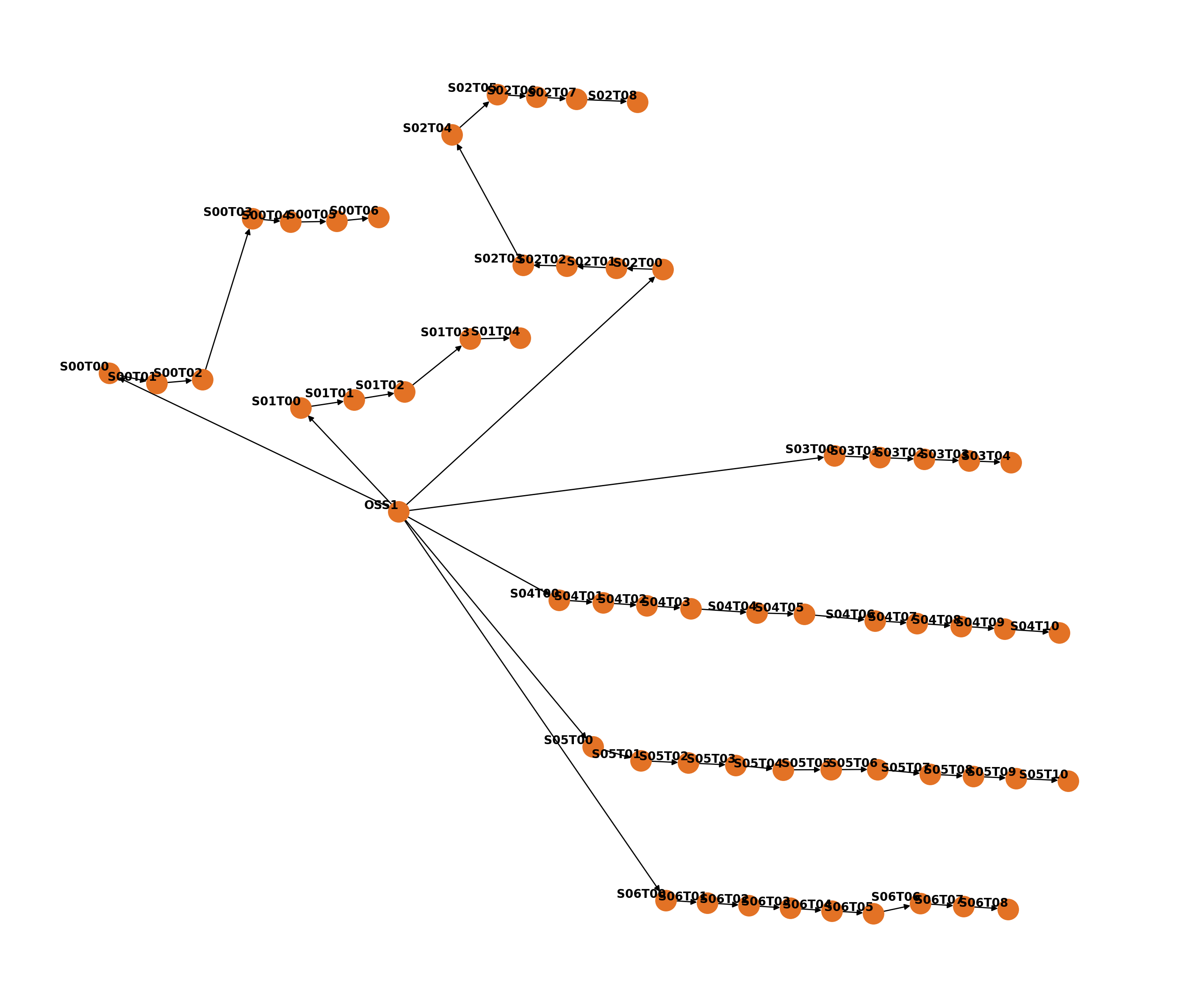
Using the plotting library, we can observe the layout for each of the farms

print(f"N turbines: {len(lbw_sim.windfarm.turbine_id)}, N substations: {len(lbw_sim.windfarm.substation_id)}")
plot.plot_farm_layout(lbw_sim.windfarm)

N turbines: 57, N substations: 1

print(f"N turbines: {len(osw_fixed_sim.windfarm.turbine_id)}, N substations: {len(osw_fixed_sim.windfarm.substation_id)}")
plot.plot_farm_layout(osw_fixed_sim.windfarm)

N turbines: 50, N substations: 1

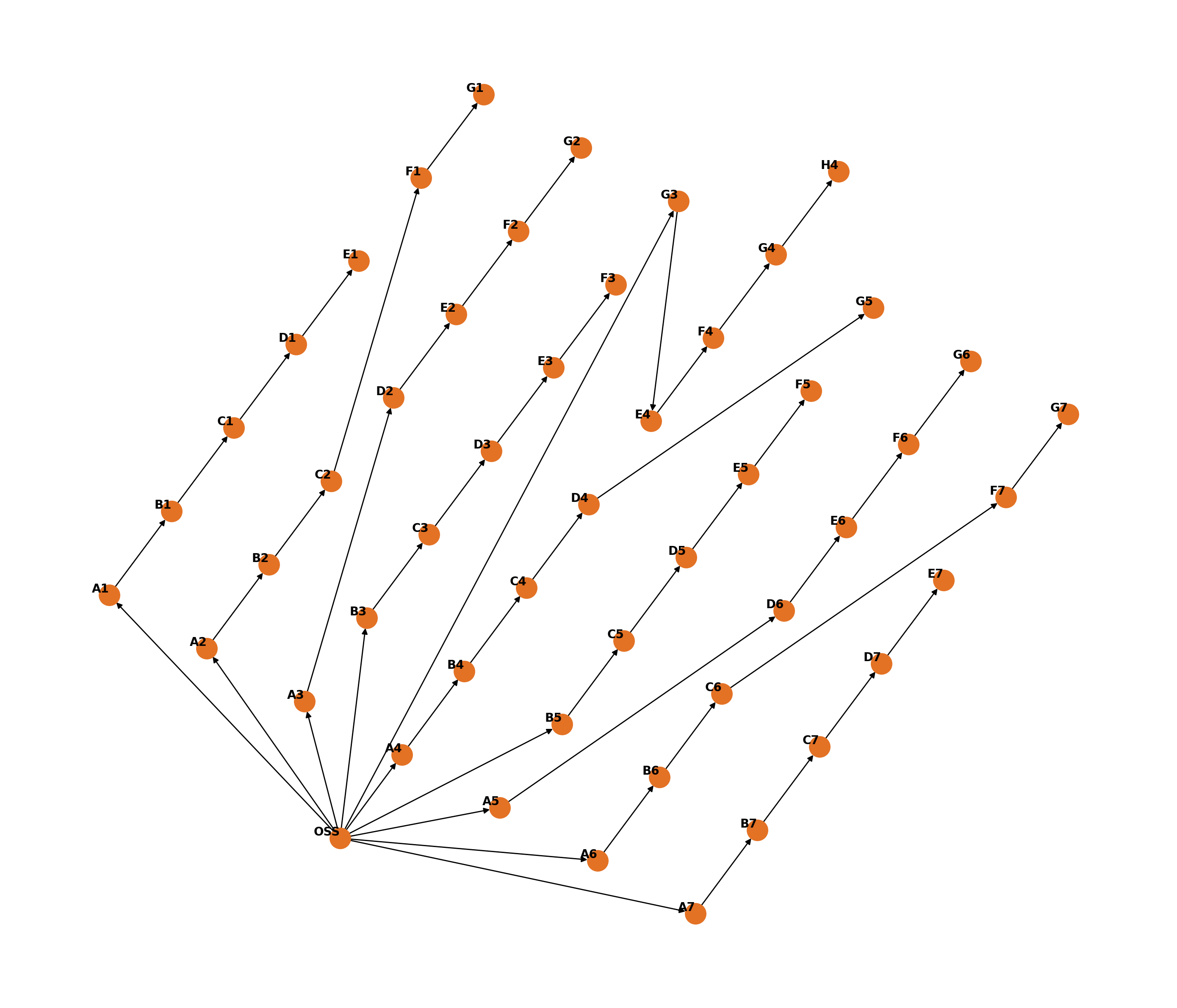
print(f"N turbines: {len(osw_floating_sim.windfarm.turbine_id)}, N substations: {len(osw_floating_sim.windfarm.substation_id)}")
plot.plot_farm_layout(osw_floating_sim.windfarm)

N turbines: 50, N substations: 1

Run the simulations

Now we can run all three simulations, delete the simulation log files, and view the run time for each simulation.

start = perf_counter()
lbw_sim.run(delete_logs=True, save_metrics_inputs=False)
run_time = perf_counter() - start
print(f"Run time: {run_time // 60} minutes {run_time % 60:.1f} seconds")

start = perf_counter()
osw_fixed_sim.run(delete_logs=True, save_metrics_inputs=False)
run_time = perf_counter() - start
print(f"Run time: {run_time // 60} minutes {run_time % 60:.1f} seconds")

start = perf_counter()
osw_floating_sim.run(delete_logs=True, save_metrics_inputs=False)
run_time = perf_counter() - start
print(f"Run time: {run_time // 60} minutes {run_time % 60:.1f} seconds")

Run time: 1.0 minutes 1.1 seconds
Run time: 1.0 minutes 3.3 seconds
Run time: 1.0 minutes 10.3 seconds

Gather the results

First we will simplify the process of getting results, ensure that all simulations are 20 years, and gather the capacities.

metrics_lbw = lbw_sim.metrics
metrics_osw_fixed = osw_fixed_sim.metrics
metrics_osw_floating = osw_floating_sim.metrics

years_check = (
    lbw_sim.env.simulation_years,
    osw_fixed_sim.env.simulation_years,
    osw_floating_sim.env.simulation_years
)
print(f"All are 20 years: {all(x == 20 for x in years_check)}")
years = 20

capacities = [  # MW
    metrics_lbw.project_capacity,
    metrics_osw_fixed.project_capacity,
    metrics_osw_floating.project_capacity,
]

columns = ["Metric", "Units", "Land-Based", "OSW-Fixed", "OSW-Floating"]
sort_order = [
    "Project Capacity",
    "Production Based Availability",
    "Total OpEx",
    "Materials",
    "Direct Labor",
    "Port Fees",
    "Fixed Costs (operations, indirect labor, etc.)",
    "Service Equipment",
    "Truck 1",
    "Truck 2",
    "Truck 3",
    "Crawler Crane - 1350 tonnes",
    "Crew Transfer Vessel 1",
    "Crew Transfer Vessel 2",
    "Crew Transfer Vessel 3",
    "Cable Laying Vessel",
    "Diving Support Vessel",
    "Heavy Lift Vessel",
    "Anchor Handling Tug",
    "Tugboat 1",
    "Tugboat 2",
]

All are 20 years: True

Now, we can gather some of the high level availability and cost statistics for each of the base scenarios.

capacity = pd.DataFrame([["Project Capacity", "MW"] + capacities], columns=columns).set_index(["Metric", "Units"])

availability = [
    "Production Based Availability",
    "%",
    metrics_lbw.production_based_availability("project", "windfarm").squeeze() * 100,
    metrics_osw_fixed.production_based_availability("project", "windfarm").squeeze() * 100,
    metrics_osw_floating.production_based_availability("project", "windfarm").squeeze() * 100,
]
availability = pd.DataFrame([availability], columns=columns).set_index(["Metric", "Units"])

opex = (
    metrics_lbw.opex("project", "windfarm").rename({0: "Land-Based"}).T
    .join(metrics_osw_fixed.opex("project", "windfarm").rename({0: "OSW-Fixed"}).T)
    .join(metrics_osw_floating.opex("project", "windfarm").rename({0: "OSW-Floating"}).T)
    / years
    / (np.array(capacities) * 1000)
)
opex.index = [
    "Fixed Costs (operations, indirect labor, etc.)",
    "Port Fees",
    "Service Equipment",
    "Direct Labor",
    "Materials",
    "Total OpEx"
]
opex["Units"] = "$/kw/yr"
opex = opex.set_index("Units", append=True).iloc[::-1]

equipment = (
    metrics_lbw.equipment_costs("project", by_equipment=True).rename({0: "Land-Based"}).T
    .join(metrics_osw_fixed.equipment_costs("project", by_equipment=True).rename({0: "OSW-Fixed"}).T, how="outer")
    .join(metrics_osw_floating.equipment_costs("project", by_equipment=True).rename({0: "OSW-Floating"}).T, how="outer")
    .fillna(0.0)
    / years
    / (np.array(capacities) * 1000)
)
equipment["Units"] = "$/kw/yr"
equipment = equipment.set_index("Units", append=True)

/tmp/ipykernel_2336/2109753505.py:5: FutureWarning: Downcasting object dtype arrays on .fillna, .ffill, .bfill is deprecated and will change in a future version. Call result.infer_objects(copy=False) instead. To opt-in to the future behavior, set `pd.set_option('future.no_silent_downcasting', True)`
  .fillna(0.0)

With each of the core costs gathered, we can combine them into a single DataFrame and view them.

results = pd.concat([capacity, availability, opex, equipment]).loc[sort_order]
results

		Land-Based	OSW-Fixed	OSW-Floating
	Units
Project Capacity	MW	199.50	600.00	600.00
Production Based Availability	%	97.44	93.79	92.52
Total OpEx	$/kw/yr	35.73	122.82	145.91
Materials	$/kw/yr	1.66	2.24	3.39
Direct Labor	$/kw/yr	0.00	0.00	0.00
Port Fees	$/kw/yr	0.00	0.50	16.74
Fixed Costs (operations, indirect labor, etc.)	$/kw/yr	18.81	47.38	50.94
Service Equipment	$/kw/yr	15.25	72.70	74.84
Truck 1	$/kw/yr	0.04	0.00	0.00
Truck 2	$/kw/yr	0.04	0.00	0.00
Truck 3	$/kw/yr	0.04	0.00	0.00
Crawler Crane - 1350 tonnes	$/kw/yr	15.13	0.00	0.00
Crew Transfer Vessel 1	$/kw/yr	0.00	1.95	1.95
Crew Transfer Vessel 2	$/kw/yr	0.00	1.95	1.95
Crew Transfer Vessel 3	$/kw/yr	0.00	1.95	1.95
Cable Laying Vessel	$/kw/yr	0.00	13.91	22.87
Diving Support Vessel	$/kw/yr	0.00	1.00	2.49
Heavy Lift Vessel	$/kw/yr	0.00	51.94	0.00
Anchor Handling Tug	$/kw/yr	0.00	0.00	4.52
Tugboat 1	$/kw/yr	0.00	0.00	19.91
Tugboat 2	$/kw/yr	0.00	0.00	19.21